Skip to content

블로그

파이썬으로 Maximum Drawdown (MDD) 확인하기

Maximum Drawdown (MDD)는 특정 기간동안 발생한 최대 낙폭을 의미하는 하방 리스크 지표 입니다. MDD가 클수록 투자 리스크가 크기 때문에 유의해야 합니다.

MDD = (기간 동안의 최저점 - 기간 동안의 최고점) / 기간 동안의 최고점으로 간단히 구할 수 있습니다.

파이썬에서 MDD를 다음과 같이 구할 수 있습니다.

import numpy as np
def get_mdd(x):
"""
MDD(Maximum Draw-Down)
:return: (peak_upper, peak_lower, mdd rate)
"""
arr_v = np.array(x)
peak_lower = np.argmax(np.maximum.accumulate(arr_v) - arr_v)
peak_upper = np.argmax(arr_v[:peak_lower])
return peak_upper, peak_lower, (arr_v[peak_lower] - arr_v[peak_upper]) / arr_v[peak_upper]
data = [['20190219', 125000.0, 127500.0, 123500.0, 126000.0, 57757], ['20190220', 125000.0, 127000.0, 124500.0, 126000.0, 68453], ['20190221', 125500.0, 126000.0, 124000.0, 125000.0, 43961], ['20190222', 125000.0, 125000.0, 123500.0, 125000.0, 31065], ['20190225', 125500.0, 126000.0, 124000.0, 125500.0, 45852], ['20190226', 125000.0, 127000.0, 124500.0, 126500.0, 37404], ['20190227', 126500.0, 127000.0, 124500.0, 126000.0, 36131], ['20190228', 126500.0, 127000.0, 124500.0, 125000.0, 69474], ['20190304', 124500.0, 125500.0, 122500.0, 123500.0, 65517], ['20190305', 123000.0, 125000.0, 122000.0, 124500.0, 35186], ['20190306', 124000.0, 124500.0, 122500.0, 123500.0, 35449], ['20190307', 123500.0, 124000.0, 122000.0, 123500.0, 34768], ['20190308', 122500.0, 122500.0, 120500.0, 121500.0, 35118], ['20190311', 121500.0, 122500.0, 120000.0, 122500.0, 39576], ['20190312', 123000.0, 124000.0, 122000.0, 123500.0, 24117], ['20190313', 123000.0, 123500.0, 121500.0, 123500.0, 37649], ['20190314', 123000.0, 124000.0, 122000.0, 123500.0, 95132], ['20190315', 123000.0, 128000.0, 123000.0, 126500.0, 107246], ['20190318', 127000.0, 131000.0, 126500.0, 131000.0, 74644], ['20190319', 130000.0, 134000.0, 129500.0, 133000.0, 68348], ['20190320', 132000.0, 133000.0, 129500.0, 131000.0, 42697], ['20190321', 130000.0, 132000.0, 127500.0, 128500.0, 54018], ['20190322', 127500.0, 129500.0, 126500.0, 127000.0, 32380], ['20190325', 125500.0, 126500.0, 124000.0, 124500.0, 37185], ['20190326', 124500.0, 125500.0, 123500.0, 124000.0, 45161], ['20190327', 124000.0, 125000.0, 123500.0, 124000.0, 34336], ['20190328', 124000.0, 124500.0, 120500.0, 121500.0, 43518], ['20190329', 122500.0, 125000.0, 122000.0, 124500.0, 39035], ['20190401', 124000.0, 126500.0, 124000.0, 126500.0, 22463], ['20190402', 125500.0, 126500.0, 123500.0, 126000.0, 31754], ['20190403', 124500.0, 128000.0, 124500.0, 128000.0, 36250], ['20190404', 128500.0, 128500.0, 126000.0, 128000.0, 34854], ['20190405', 127500.0, 129000.0, 126000.0, 127500.0, 33513], ['20190408', 127500.0, 128000.0, 126000.0, 128000.0, 39005], ['20190409', 128000.0, 129000.0, 127500.0, 128500.0, 33266], ['20190410', 128000.0, 129000.0, 126500.0, 128000.0, 64476], ['20190411', 128500.0, 129000.0, 125000.0, 125000.0, 84802], ['20190412', 126000.0, 127500.0, 125500.0, 127000.0, 39663], ['20190415', 126500.0, 128500.0, 126000.0, 127000.0, 61140], ['20190416', 127000.0, 129000.0, 126500.0, 128500.0, 40123], ['20190417', 128500.0, 129000.0, 127000.0, 128000.0, 30846], ['20190418', 128000.0, 128500.0, 124000.0, 124500.0, 55346], ['20190419', 124500.0, 125000.0, 122000.0, 123000.0, 53439], ['20190422', 123000.0, 123500.0, 121000.0, 122500.0, 30421], ['20190423', 122500.0, 123500.0, 120500.0, 121500.0, 54997], ['20190424', 122500.0, 122500.0, 119500.0, 120000.0, 63486], ['20190425', 121000.0, 121000.0, 118500.0, 119000.0, 36046], ['20190426', 118500.0, 119500.0, 117000.0, 119000.0, 43749], ['20190429', 119000.0, 119500.0, 117000.0, 119500.0, 33516], ['20190430', 122000.0, 123000.0, 119000.0, 119500.0, 94118], ['20190502', 118500.0, 122000.0, 118000.0, 121000.0, 56723], ['20190503', 121000.0, 122000.0, 119500.0, 120000.0, 35240], ['20190507', 118500.0, 119500.0, 117000.0, 117500.0, 44453], ['20190508', 116500.0, 117000.0, 115000.0, 116500.0, 52805], ['20190509', 117000.0, 117000.0, 113000.0, 113000.0, 116012], ['20190510', 113000.0, 114500.0, 110000.0, 111500.0, 86072], ['20190513', 110500.0, 110500.0, 107500.0, 108500.0, 70847], ['20190514', 107500.0, 108000.0, 105000.0, 106500.0, 92820], ['20190515', 107000.0, 107500.0, 105000.0, 107000.0, 68937], ['20190516', 107000.0, 107500.0, 104000.0, 105000.0, 64047]]
import pandas as pd
df = pd.DataFrame(data, columns=['date', 'open', 'high', 'low', 'close', 'volume'])
mdd = get_mdd(df['close'])
(19, 59, -0.21052631578947367)
import matplotlib.pyplot as plt
import matplotlib.gridspec as gridspec
fig = plt.figure(figsize=(8, 5))
fig.set_facecolor('w')
gs = gridspec.GridSpec(2, 1, height_ratios=[3, 1])
axes = []
axes.append(plt.subplot(gs[0]))
axes.append(plt.subplot(gs[1], sharex=axes[0]))
axes[0].get_xaxis().set_visible(False)
from mpl_finance import candlestick_ohlc
x = np.arange(len(df.index))
ohlc = df[['open', 'high', 'low', 'close']].astype(int).values
dohlc = np.hstack((np.reshape(x, (-1, 1)), ohlc))
# 봉차트
candlestick_ohlc(axes[0], dohlc, width=0.5, colorup='r', colordown='b')
# 거래량 차트
axes[1].bar(x, df.volume, color='k', width=0.6, align='center')
import datetime
_xticks = []
_xlabels = []
_wd_prev = 0
for _x, d in zip(x, df.date.values):
weekday = datetime.datetime.strptime(str(d), '%Y%m%d').weekday()
if weekday <= _wd_prev:
_xticks.append(_x)
_xlabels.append(datetime.datetime.strptime(str(d), '%Y%m%d').strftime('%m/%d'))
_wd_prev = weekday
axes[1].set_xticks(_xticks)
axes[1].set_xticklabels(_xlabels, rotation=45, minor=False)
# MDD 그리기
axes[0].plot(mdd[:2], df.loc[mdd[:2], 'close'], 'k')
plt.tight_layout()
plt.show()

mdd

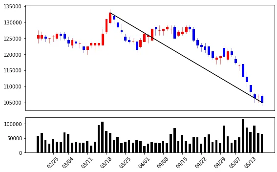
이 차트에서는 약 -21%의 MDD가 발생했습니다. 포트폴리오를 구성할 때 보유하고자 하는 종목들의 MDD를 전체적으로 확인해보는 것이 좋습니다. 특히 보유하고자 하는 종목 수가 적을수록 MDD가 낮은 종목을 보유하는 것이 안전할 것입니다.
IMF에서 GDP 관련 지표를 파이썬으로 얻어오기

IMF에서 세계 지표들을 확인할 수 있습니다. 이번 포스트에서는 파이썬으로 IMF 사이트에서 GDP 관련 지표들을 파이썬으로 얻어오는 방법을 다루겠습니다.

국제통화기금(IMF, International Monetary Fund)는 선진국들이 출자하는 펀드이며 세계 경제 지표를 조사하여 공개하고 있습니다. IMF에 대한 자세한 사항은 나무위키 - IMF를 참고하세요.

국내총생산(GDP, Gross Domestic Product)에는 명목 GDP(Nominal GDP)와 실질 GDP(Real GDP)가 있습니다. 명목 GDP는 당해의 시장가격으로 가치를 계산하고 실질 GDP는 물가를 고려한 가격으로 가치를 계산합니다. 따라서 경제성장률은 실질 GDP의 성장률을 의미합니다. 한국의 GDP는 나라지표 사이트에서 확인할 수 있습니다.

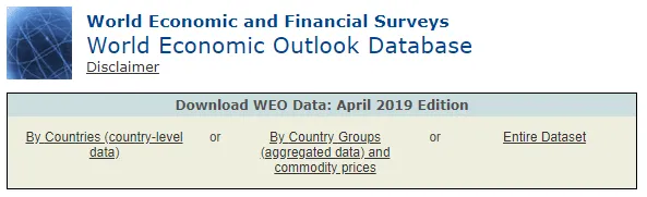
한국 뿐만 아니라 세계 주요 국가들의 GDP 관련 지표들을 확인해 보겠습니다. IMF - World Econimic Outlook Databases에서 최신 발표 내용을 확인하면 됩니다.

먼저 By Countries (country-level data)를 선택합니다.

imf weo

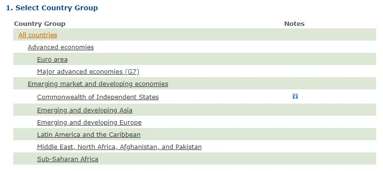
그리고 데이터를 얻고자 하는 국가를 선택합니다. 여기서는 모든 국가를 선택하겠습니다.

imf weo

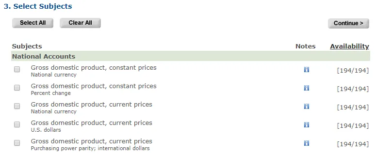
다음으로 얻고자 하는 데이터 종류를 선택합니다. 이 포스트에서 확인하고자 하는 데이터는 Gross domestic product, constant prices (Percent change)Output gap in percent of potential GDP (Percent of potential GDP)이긴 하지만 전체 다 선택하겠습니다.

imf weo

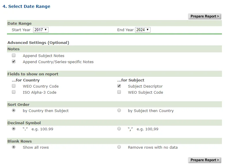
이제 다음 화면에서 Start Year를 1980으로 변경하고 나머지는 기본 설정으로 둔 상태에서 Prepare Report 버튼을 누릅니다.

imf weo

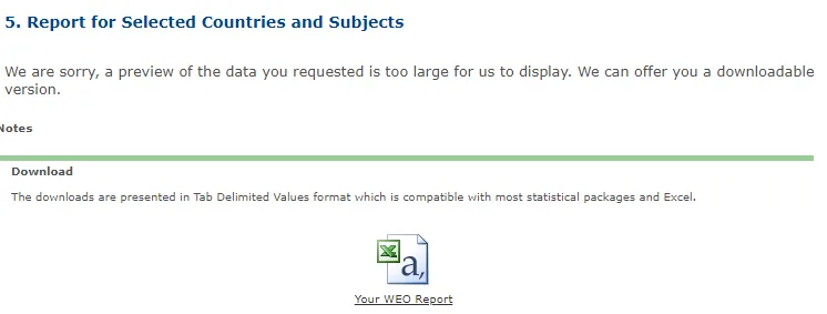
조금 기다리면 다음과 같은 화면이 나옵니다. 화면에 표시하기에 데이터가 너무 크다는 문구가 나오는데, 그 아래에 다운로드 링크가 있습니다. 이 링크를 클릭하면 WEO_Data.xls 파일을 다운받을 수 있습니다. 이 파일은 사실 TSV(Tab-separated Values) 입니다.

imf weo

이제 파이썬으로 이 파일을 다운받고 읽어 보겠습니다. 먼저 다음처럼 requests 라이브러리를 사용해서 IMF 데이터를 요청하고 파일을 저장합니다.

import requests
url = 'https://www.imf.org/external/pubs/ft/weo/2019/01/weodata/weoreptc.aspx?pr.x=49&pr.y=15&sy=1980&ey=2024&scsm=1&ssd=1&sort=country&ds=.&br=1&c=512%2C668%2C914%2C672%2C612%2C946%2C614%2C137%2C311%2C546%2C213%2C674%2C911%2C676%2C314%2C548%2C193%2C556%2C122%2C678%2C912%2C181%2C313%2C867%2C419%2C682%2C513%2C684%2C316%2C273%2C913%2C868%2C124%2C921%2C339%2C948%2C638%2C943%2C514%2C686%2C218%2C688%2C963%2C518%2C616%2C728%2C223%2C836%2C516%2C558%2C918%2C138%2C748%2C196%2C618%2C278%2C624%2C692%2C522%2C694%2C622%2C962%2C156%2C142%2C626%2C449%2C628%2C564%2C228%2C565%2C924%2C283%2C233%2C853%2C632%2C288%2C636%2C293%2C634%2C566%2C238%2C964%2C662%2C182%2C960%2C359%2C423%2C453%2C935%2C968%2C128%2C922%2C611%2C714%2C321%2C862%2C243%2C135%2C248%2C716%2C469%2C456%2C253%2C722%2C642%2C942%2C643%2C718%2C939%2C724%2C734%2C576%2C644%2C936%2C819%2C961%2C172%2C813%2C132%2C726%2C646%2C199%2C648%2C733%2C915%2C184%2C134%2C524%2C652%2C361%2C174%2C362%2C328%2C364%2C258%2C732%2C656%2C366%2C654%2C144%2C336%2C146%2C263%2C463%2C268%2C528%2C532%2C923%2C944%2C738%2C176%2C578%2C534%2C537%2C536%2C742%2C429%2C866%2C433%2C369%2C178%2C744%2C436%2C186%2C136%2C925%2C343%2C869%2C158%2C746%2C439%2C926%2C916%2C466%2C664%2C112%2C826%2C111%2C542%2C298%2C967%2C927%2C443%2C846%2C917%2C299%2C544%2C582%2C941%2C474%2C446%2C754%2C666%2C698&s=NGDP_R%2CNGDP_RPCH%2CNGDP%2CNGDPD%2CPPPGDP%2CNGDP_D%2CNGDPRPC%2CNGDPRPPPPC%2CNGDPPC%2CNGDPDPC%2CPPPPC%2CNGAP_NPGDP%2CPPPSH%2CPPPEX%2CNID_NGDP%2CNGSD_NGDP%2CPCPI%2CPCPIPCH%2CPCPIE%2CPCPIEPCH%2CFLIBOR6%2CTM_RPCH%2CTMG_RPCH%2CTX_RPCH%2CTXG_RPCH%2CLUR%2CLE%2CLP%2CGGR%2CGGR_NGDP%2CGGX%2CGGX_NGDP%2CGGXCNL%2CGGXCNL_NGDP%2CGGSB%2CGGSB_NPGDP%2CGGXONLB%2CGGXONLB_NGDP%2CGGXWDN%2CGGXWDN_NGDP%2CGGXWDG%2CGGXWDG_NGDP%2CNGDP_FY%2CBCA%2CBCA_NGDPD&grp=0&a='
res = requests.get(url)
if res.status_code == 200:
with open('data/2019-06-09-imf_gdp/WEO_Data_2019.xls', 'wb') as fout:
fout.write(res.content)

그리고 저장된 파일을 pandas 라이브러리를 사용하여 읽고 활용합니다. 확장자가 xls이기는 하지만 실제 내용은 TSV 형태이므로 read_csv() 함수를 사용할 수 있습니다.

그리고 저장된 파일을 pandas 라이브러리를 사용하여 읽고 활용합니다. 확장자가 xls이기는 하지만 실제 내용은 TSV 형태이므로 read_csv() 함수를 사용할 수 있습니다.

import pandas as pd
df = pd.read_csv('data/2019-06-09-imf_gdp/WEO_Data_2019.xls', sep='\t', encoding='ISO-8859-1')
df.head()
CountrySubject DescriptorUnitsScaleCountry/Series-specific Notes19801981198219831984201620172018201920202021202220232024Estimates Start After
AfghanistanGross domestic product, constant pricesNational currencyBillionsSource: National Statistics Office Latest actu…NaNNaNNaNNaNNaN493.073506.215517.858533.394552.063574.127599.933629.880664.4522017.0
AfghanistanGross domestic product, constant pricesPercent changeNaNSee notes for: Gross domestic product, consta…NaNNaNNaNNaNNaN2.1642.6652.3003.0003.5003.9974.4954.9925.4892017.0
AfghanistanGross domestic product, current pricesNational currencyBillionsSource: National Statistics Office Latest actu…NaNNaNNaNNaNNaN1,318.4781,377.5351,418.1281,488.8611,595.0531,733.5391,902.1092,096.9512,322.6502017.0
AfghanistanGross domestic product, current pricesU.S. dollarsBillionsSee notes for: Gross domestic product, curren…NaNNaNNaNNaNNaN19.42820.23519.58519.99020.68221.92823.57725.45027.6082017.0
AfghanistanGross domestic product, current pricesPurchasing power parity; international dollarsBillionsSee notes for: Gross domestic product, curren…NaNNaNNaNNaNNaN66.38469.44972.64876.15880.47085.42691.11397.643105.1582017.0

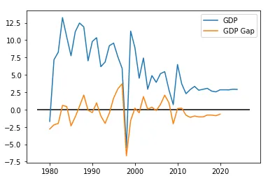
여기서 한국의 GDP 성장률과 GDP Gap 데이터만 뽑아서 차트로 가시화해보면 다음과 같습니다.

df_gdp = df[(df['Country'] == 'Korea') & (df['Subject Descriptor'] == 'Gross domestic product, constant prices') & (df['Units'] == 'Percent change')].iloc[:, 5:-1]
df_gdpgap = df[(df['Country'] == 'Korea') & (df['Subject Descriptor'] == 'Output gap in percent of potential GDP') & (df['Units'] == 'Percent of potential GDP')].iloc[:, 5:-1]
x_gdp = df_gdp.columns.astype(int)
y_gdp = df_gdp.values[0].astype(float)
x_gdpgap = df_gdpgap.columns.astype(int)
y_gdpgap = df_gdpgap.values[0].astype(float)
import matplotlib.pyplot as plt
import matplotlib
%matplotlib inline
plt.plot(x_gdp, y_gdp, label='GDP')
plt.plot(x_gdpgap, y_gdpgap, label='GDP Gap')
plt.hlines(0, xmin=x_gdp[0]-3, xmax=x_gdp[-1]+3)
plt.legend()

res

bokeh로 봉차트(Candlestick Chart) 그리기

파이썬에서 봉차트를 제공하는 라이브러리가 많지 않습니다. 필자는 matplotlib에서 떨어져 나온 mpl_finance와 bokeh 정도로 알고 있습니다. 이미 mpl_finance로 봉차트를 그리는 방법은 이전 포스트 Matplotlib으로 봉차트(Candlestick Chart) 그리기 에서 다루었습니다.

이번 포스트에서 bokeh로 봉차트를 그리는 방법에 대해서 다루겠습니다. bokeh는 Anaconda에서 개발 중인 차트 라이브러리 입니다. matplotlib과 matplotlib 기반인 seaborn과는 다르게 독자 노선을 가지는 라이브러리 입니다. bokeh는 웹에 최적화 되어있는 라이브러리 입니다. matplotlib을 웹브라우저에 띄우려면 차트를 png 등의 그림으로 변환하여 보여줘야 해서 응답형(reponsible) 차트를 웹에 띄우기가 어렵습니다. 그래서 보통 웹에 차트를 띄울 때는 데이터만 서버에서 받고 Chart.jsD3.js 같은 자바스크립트 라이브러리를 사용하여 데이터를 가시화 합니다. bokeh는 파이썬에서 차트를 가시화하고 그 결과를 쉽게 웹에 띄울 수 있는 여러 방법을 제공합니다. 이 포스트에서는 다루지 않겠습니다.

bokeh에서 봉차트를 제공하고 있습니다. bokeh 봉차트 문서에서 상세한 정보를 확인해 보세요.

먼저 Anaconda3가 설치되어 있는 상태라 가정하고 글을 이어나가겠습니다. Jupyter Lab(Notebook)에서 bokeh가 잘 설치되어 있는지 확인합니다.

from bokeh.io import output_notebook, show
from bokeh.plotting import figure, gridplot
output_notebook()

BokehJS 0.12.16 successfully loaded.

이렇게 로딩이 성공되었다는 메시지가 뜨는지 확인합니다. 만약 다음과 같은 메시지가 뜬다면 Jupyter Lab의 Extension을 설치해야 합니다.

Loading BokehJS ...
JavaScript output is disabled in JupyterLab

Anaconda Prompt에서 다음과 같이 jupyterlab_bokeh 확장을 설치합니다.

Terminal window
jupyter labextension install jupyterlab_bokeh

설치가 되지 않는다면 아마도 node.js가 설치되어 있지 않아서일 것입니다. 그렇다면 conda install nodejs를 통해 먼저 node.js를 설치하고 다시 jupyterlab_bokeh 확장을 설치합니다.

bokeh가 잘 설치되어 있다면 이제 봉차트를 그릴 준비가 되었습니다. 차트 데이터는 다음과 같이 ['date', 'open', 'high', 'low', 'close', 'volume']의 리스트로 있습니다.

import pandas as pd
data = [['20190219', 125000.0, 127500.0, 123500.0, 126000.0, 57757], ['20190220', 125000.0, 127000.0, 124500.0, 126000.0, 68453], ['20190221', 125500.0, 126000.0, 124000.0, 125000.0, 43961], ['20190222', 125000.0, 125000.0, 123500.0, 125000.0, 31065], ['20190225', 125500.0, 126000.0, 124000.0, 125500.0, 45852], ['20190226', 125000.0, 127000.0, 124500.0, 126500.0, 37404], ['20190227', 126500.0, 127000.0, 124500.0, 126000.0, 36131], ['20190228', 126500.0, 127000.0, 124500.0, 125000.0, 69474], ['20190304', 124500.0, 125500.0, 122500.0, 123500.0, 65517], ['20190305', 123000.0, 125000.0, 122000.0, 124500.0, 35186], ['20190306', 124000.0, 124500.0, 122500.0, 123500.0, 35449], ['20190307', 123500.0, 124000.0, 122000.0, 123500.0, 34768], ['20190308', 122500.0, 122500.0, 120500.0, 121500.0, 35118], ['20190311', 121500.0, 122500.0, 120000.0, 122500.0, 39576], ['20190312', 123000.0, 124000.0, 122000.0, 123500.0, 24117], ['20190313', 123000.0, 123500.0, 121500.0, 123500.0, 37649], ['20190314', 123000.0, 124000.0, 122000.0, 123500.0, 95132], ['20190315', 123000.0, 128000.0, 123000.0, 126500.0, 107246], ['20190318', 127000.0, 131000.0, 126500.0, 131000.0, 74644], ['20190319', 130000.0, 134000.0, 129500.0, 133000.0, 68348], ['20190320', 132000.0, 133000.0, 129500.0, 131000.0, 42697], ['20190321', 130000.0, 132000.0, 127500.0, 128500.0, 54018], ['20190322', 127500.0, 129500.0, 126500.0, 127000.0, 32380], ['20190325', 125500.0, 126500.0, 124000.0, 124500.0, 37185], ['20190326', 124500.0, 125500.0, 123500.0, 124000.0, 45161], ['20190327', 124000.0, 125000.0, 123500.0, 124000.0, 34336], ['20190328', 124000.0, 124500.0, 120500.0, 121500.0, 43518], ['20190329', 122500.0, 125000.0, 122000.0, 124500.0, 39035], ['20190401', 124000.0, 126500.0, 124000.0, 126500.0, 22463], ['20190402', 125500.0, 126500.0, 123500.0, 126000.0, 31754], ['20190403', 124500.0, 128000.0, 124500.0, 128000.0, 36250], ['20190404', 128500.0, 128500.0, 126000.0, 128000.0, 34854], ['20190405', 127500.0, 129000.0, 126000.0, 127500.0, 33513], ['20190408', 127500.0, 128000.0, 126000.0, 128000.0, 39005], ['20190409', 128000.0, 129000.0, 127500.0, 128500.0, 33266], ['20190410', 128000.0, 129000.0, 126500.0, 128000.0, 64476], ['20190411', 128500.0, 129000.0, 125000.0, 125000.0, 84802], ['20190412', 126000.0, 127500.0, 125500.0, 127000.0, 39663], ['20190415', 126500.0, 128500.0, 126000.0, 127000.0, 61140], ['20190416', 127000.0, 129000.0, 126500.0, 128500.0, 40123], ['20190417', 128500.0, 129000.0, 127000.0, 128000.0, 30846], ['20190418', 128000.0, 128500.0, 124000.0, 124500.0, 55346], ['20190419', 124500.0, 125000.0, 122000.0, 123000.0, 53439], ['20190422', 123000.0, 123500.0, 121000.0, 122500.0, 30421], ['20190423', 122500.0, 123500.0, 120500.0, 121500.0, 54997], ['20190424', 122500.0, 122500.0, 119500.0, 120000.0, 63486], ['20190425', 121000.0, 121000.0, 118500.0, 119000.0, 36046], ['20190426', 118500.0, 119500.0, 117000.0, 119000.0, 43749], ['20190429', 119000.0, 119500.0, 117000.0, 119500.0, 33516], ['20190430', 122000.0, 123000.0, 119000.0, 119500.0, 94118], ['20190502', 118500.0, 122000.0, 118000.0, 121000.0, 56723], ['20190503', 121000.0, 122000.0, 119500.0, 120000.0, 35240], ['20190507', 118500.0, 119500.0, 117000.0, 117500.0, 44453], ['20190508', 116500.0, 117000.0, 115000.0, 116500.0, 52805], ['20190509', 117000.0, 117000.0, 113000.0, 113000.0, 116012], ['20190510', 113000.0, 114500.0, 110000.0, 111500.0, 86072], ['20190513', 110500.0, 110500.0, 107500.0, 108500.0, 70847], ['20190514', 107500.0, 108000.0, 105000.0, 106500.0, 92820], ['20190515', 107000.0, 107500.0, 105000.0, 107000.0, 68937], ['20190516', 107000.0, 107500.0, 104000.0, 105000.0, 64047]]
df = pd.DataFrame(data, columns=['date', 'open', 'high', 'low', 'close', 'volume'])
dateopenhighlowclosevolume
20190219125000.0127500.0123500.0126000.057757
20190220125000.0127000.0124500.0126000.068453
20190221125500.0126000.0124000.0125000.043961
20190222125000.0125000.0123500.0125000.031065
20190225125500.0126000.0124000.0125500.045852
20190226125000.0127000.0124500.0126500.037404
20190227126500.0127000.0124500.0126000.036131
20190228126500.0127000.0124500.0125000.069474
20190304124500.0125500.0122500.0123500.065517
20190305123000.0125000.0122000.0124500.035186
20190306124000.0124500.0122500.0123500.035449
20190307123500.0124000.0122000.0123500.034768
20190308122500.0122500.0120500.0121500.035118
20190311121500.0122500.0120000.0122500.039576
20190312123000.0124000.0122000.0123500.024117
20190313123000.0123500.0121500.0123500.037649
20190314123000.0124000.0122000.0123500.095132
20190315123000.0128000.0123000.0126500.0107246
20190318127000.0131000.0126500.0131000.074644
20190319130000.0134000.0129500.0133000.068348
20190320132000.0133000.0129500.0131000.042697
20190321130000.0132000.0127500.0128500.054018
20190322127500.0129500.0126500.0127000.032380
20190325125500.0126500.0124000.0124500.037185
20190326124500.0125500.0123500.0124000.045161
20190327124000.0125000.0123500.0124000.034336
20190328124000.0124500.0120500.0121500.043518
20190329122500.0125000.0122000.0124500.039035
20190401124000.0126500.0124000.0126500.022463
20190402125500.0126500.0123500.0126000.031754
20190403124500.0128000.0124500.0128000.036250
20190404128500.0128500.0126000.0128000.034854
20190405127500.0129000.0126000.0127500.033513
20190408127500.0128000.0126000.0128000.039005
20190409128000.0129000.0127500.0128500.033266
20190410128000.0129000.0126500.0128000.064476
20190411128500.0129000.0125000.0125000.084802
20190412126000.0127500.0125500.0127000.039663
20190415126500.0128500.0126000.0127000.061140
20190416127000.0129000.0126500.0128500.040123
20190417128500.0129000.0127000.0128000.030846
20190418128000.0128500.0124000.0124500.055346
20190419124500.0125000.0122000.0123000.053439
20190422123000.0123500.0121000.0122500.030421
20190423122500.0123500.0120500.0121500.054997
20190424122500.0122500.0119500.0120000.063486
20190425121000.0121000.0118500.0119000.036046
20190426118500.0119500.0117000.0119000.043749
20190429119000.0119500.0117000.0119500.033516
20190430122000.0123000.0119000.0119500.094118
20190502118500.0122000.0118000.0121000.056723
20190503121000.0122000.0119500.0120000.035240
20190507118500.0119500.0117000.0117500.044453
20190508116500.0117000.0115000.0116500.052805
20190509117000.0117000.0113000.0113000.0116012
20190510113000.0114500.0110000.0111500.086072
20190513110500.0110500.0107500.0108500.070847
20190514107500.0108000.0105000.0106500.092820
20190515107000.0107500.0105000.0107000.068937
20190516107000.0107500.0104000.0105000.064047

bokeh를 이용해 봉차트를 그려봅니다. 먼저 데이터에서 양봉과 음봉에 대한 mask를 저장합니다.

inc = df.close >= df.open
dec = df.open > df.close

inc는 양봉, dec는 음봉에 해당합니다. 이제 봉들을 그려줍니다. 하나의 봉은 bokeh에서 segmentvbar로 구성되어 있습니다. segment는 high와 low까지 선으로 그은 봉의 꼬리를 그리는데 사용됩니다. vbar로는 봉의 몸통을 그립니다.

p_candlechart = figure(plot_width=1050, plot_height=200, x_range=(-1, len(df)), tools="crosshair")
p_candlechart.segment(df.index[inc], df.high[inc], df.index[inc], df.low[inc], color="red")
p_candlechart.segment(df.index[dec], df.high[dec], df.index[dec], df.low[dec], color="blue")
p_candlechart.vbar(df.index[inc], 0.5, df.open[inc], df.close[inc], fill_color="red", line_color="red")
p_candlechart.vbar(df.index[dec], 0.5, df.open[dec], df.close[dec], fill_color="blue", line_color="blue")

봉차트 밑에 거래량 막대차트(Bar Chart)까지 그려 줍니다. 이 때도 vbar를 사용하면 됩니다.

p_volumechart = figure(plot_width=1050, plot_height=100, x_range=p_candlechart.x_range, tools="crosshair")
p_volumechart.vbar(df.index, 0.5, df.volume, fill_color="black", line_color="black")

그리고 마지막으로 위 차트들을 gridplot으로 배치하여 가시화합니다.

p = gridplot([[p_candlechart], [p_volumechart]], toolbar_location=None)
show(p)

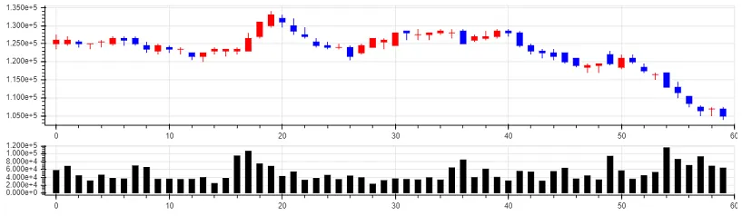
이 코드들을 모아서 다음과 같은 봉차트를 그릴 수 있습니다.

from bokeh.io import show, output_file
from bokeh.plotting import figure
from bokeh.layouts import gridplot
inc = df.close >= df.open
dec = df.open > df.close
p_candlechart = figure(plot_width=1050, plot_height=200, x_range=(-1, len(df)), tools="crosshair")
p_candlechart.segment(df.index[inc], df.high[inc], df.index[inc], df.low[inc], color="red")
p_candlechart.segment(df.index[dec], df.high[dec], df.index[dec], df.low[dec], color="blue")
p_candlechart.vbar(df.index[inc], 0.5, df.open[inc], df.close[inc], fill_color="red", line_color="red")
p_candlechart.vbar(df.index[dec], 0.5, df.open[dec], df.close[dec], fill_color="blue", line_color="blue")
p_volumechart = figure(plot_width=1050, plot_height=100, x_range=p_candlechart.x_range, tools="crosshair")
p_volumechart.vbar(df.index, 0.5, df.volume, fill_color="black", line_color="black")
p = gridplot([[p_candlechart], [p_volumechart]], toolbar_location=None)
show(p)

chart1

그러나 여기서 각 axis에 표시된 레이블들이 유용한 정보를 주지 못하고 있습니다. 좀 더 보기 좋게 레이블들을 포메팅 해보겠습니다.

p_candlechart.yaxis[0].formatter = NumeralTickFormatter(format='0,0')
p_candlechart.xaxis.visible = False

p_candlechart의 y 레이블을 다음과 같이 천단위로 콤마를 붙인 숫자로 표현합니다.

여기서 x 레이블은 거래량 차트에만 표시하기 위해서 숨기도록 합니다.

p_volumechart의 x 레이블을 날짜로 표현하고 y 레이블을 숫자로 표현합니다.

major_label = {
i: date.strftime('%Y%m%d') for i, date in enumerate(pd.to_datetime(df["date"]))
}
major_label.update({len(df): ''})
p_volumechart.xaxis.major_label_overrides = major_label
p_volumechart.yaxis[0].formatter = NumeralTickFormatter(format='0,0')

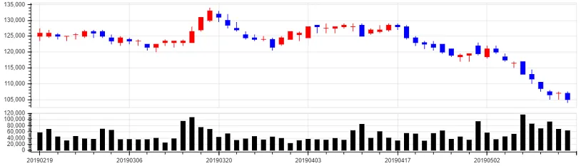
x 레이블의 마지막 값은 잘려서 나와서 숨겼습니다. 이제 이 코드들을 추가해서 다시 봉차트를 그려봅니다.

from bokeh.io import show, output_file
from bokeh.plotting import figure
from bokeh.layouts import gridplot
from bokeh.models.formatters import NumeralTickFormatter
inc = df.close >= df.open
dec = df.open > df.close
p_candlechart = figure(plot_width=1050, plot_height=200, x_range=(-1, len(df)), tools="crosshair")
p_candlechart.segment(df.index[inc], df.high[inc], df.index[inc], df.low[inc], color="red")
p_candlechart.segment(df.index[dec], df.high[dec], df.index[dec], df.low[dec], color="blue")
p_candlechart.vbar(df.index[inc], 0.5, df.open[inc], df.close[inc], fill_color="red", line_color="red")
p_candlechart.vbar(df.index[dec], 0.5, df.open[dec], df.close[dec], fill_color="blue", line_color="blue")
p_candlechart.yaxis[0].formatter = NumeralTickFormatter(format='0,0')
p_candlechart.xaxis.visible = False
p_volumechart = figure(plot_width=1050, plot_height=100, x_range=p_candlechart.x_range, tools="crosshair")
p_volumechart.vbar(df.index, 0.5, df.volume, fill_color="black", line_color="black")
major_label = {
i: date.strftime('%Y%m%d') for i, date in enumerate(pd.to_datetime(df["date"]))
}
major_label.update({len(df): ''})
p_volumechart.xaxis.major_label_overrides = major_label
p_volumechart.yaxis[0].formatter = NumeralTickFormatter(format='0,0')
p = gridplot([[p_candlechart], [p_volumechart]], toolbar_location=None)
show(p)

chart2

이렇게 x축은 날짜가, y축은 숫자가 보기좋게 나오게 됩니다. 이 차트를 html, json 등으로 웹에 넣어줄 수 있습니다. 자세한 사항은 bokeh 문서 Embedding Plots and Apps를 확인해 주세요.

아나콘다(Anaconda) 32bit 환경 설치하기

아나콘다는 파이썬 및 데이터 과학(data science) 패키지가 포함된 배포판 입니다. 기본적으로 아나콘다는 64bit 버전을 제공하고 있습니다.

anaconda

그러나 시스템 트레이딩과 같이 Windows 환경에서 다른 프로그램들과 통신할 때 32bit 버전이 필요한 경우가 종종 있습니다. 이번 포스트에서는 아나콘다에서 32bit 파이썬 환경을 구성하는 방법에 대해서 다룹니다.

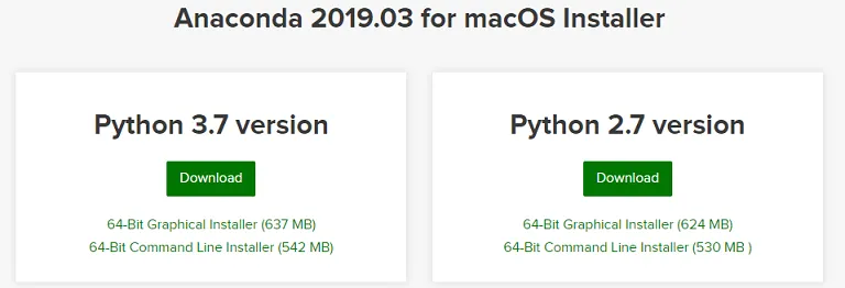
먼저 64bit 버전의 아나콘다를 다운받아서 설치합니다. 아나콘다 다운로드 페이지에서 최신 버전의 아나콘다를 받을 수 있습니다.

Anaconda Prompt를 열고 다음과 같이 명령을 입력합니다.

Terminal window
set CONDA_FORCE_32BIT=1
conda create -n py37_32 python=3.7 anaconda

설치하는데 시간이 꽤 걸릴 것이니 차분히 기다립니다. 여기서 python=3.7부분을 수정하여 원하는 버전을 설치할 수 있습니다.

설치가 완료되면 이제 32bit 버전의 파이썬을 사용할 수 있습니다. 다음과 같이 좀전에 설치한 파이썬 32bit 환경을 활성화 시키면 됩니다.

Terminal window
activate py37_32

프롬프트 커맨드 라인 처음에 (py37_32)가 표시되어 있으면 활성화가 제대로 된 것입니다. 이 환경을 비활성화 시키려면 다음과 같이 명령하면 됩니다.

Terminal window
deactivate

참고로 리눅스 운영체제에서는 source activate py37_32, source deactivate와 같이 명령을 줘야 합니다.

파이썬으로 크레온 플러스(Creon Plus) 자동 로그인하기

시스템 트레이딩에 관심 있는 분들이라면 주식투자 자동화에도 관심이 있을 것입니다. 주식투자 자동화의 첫걸음은 증권사 HTS API 자동 로그인 입니다. 증권사 HTS마다 그 방법이 다르며 이번 포스트에서는 대신증권의 크레온 플러스를 파이썬에서 자동으로 로그인하는 방법을 다루겠습니다.

크레온 다운로드센터에서 CREON HTS를 다운받습니다. CREON HTSCREON Plus가 포함되어 있습니다. 설치 과정은 생략하겠습니다.

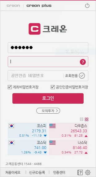
크레온 HTS를 실행하면 다음과 같은 로그인 창이 나타날 것입니다. 직접 크레온 HTS에 로그인하여 API를 사용할 때는 로그인 창 상단에 creon plus 버튼을 누르고 ID, 비밀번호, 공인인증 비밀번호(조회전용이 아닌 경우)를 입력하여 로그인 버튼을 누르면 됩니다.

크레온 로그인 창

이제 파이썬에서 크레온 HTS에 자동으로 로그인하기 위한 준비를 합니다.

파이썬 32bit 환경은 아나콘다를 설치 후에 32bit 환경을 설치하는 것을 권장합니다. 그 방법은 이 포스트를 참고 바랍니다.

커맨드 창에서 다음 pip 명령으로 pywinautopywin32를 설치합니다.

Terminal window
pip install pywinauto
pip install pywin32

크레온 API를 감싸는(wrapping) 클래스를 만들겠습니다.

import win32com.client
from pywinauto import application
class Creon:
def __init__(self):
self.obj_CpUtil_CpCybos = win32com.client.Dispatch('CpUtil.CpCybos')
def kill_client(self):
os.system('taskkill /IM coStarter* /F /T')
os.system('taskkill /IM CpStart* /F /T')
os.system('taskkill /IM DibServer* /F /T')
os.system('wmic process where "name like \'%coStarter%\'" call terminate')
os.system('wmic process where "name like \'%CpStart%\'" call terminate')
os.system('wmic process where "name like \'%DibServer%\'" call terminate')
def connect(self, id_, pwd, pwdcert):
if not self.connected():
self.disconnect()
self.kill_client()
app = application.Application()
app.start(
'C:\CREON\STARTER\coStarter.exe /prj:cp /id:{id} /pwd:{pwd} /pwdcert:{pwdcert} /autostart'.format(
id=id_, pwd=pwd, pwdcert=pwdcert
)
)
while not self.connected():
time.sleep(1)
return True
def connected(self):
b_connected = self.obj_CpUtil_CpCybos.IsConnect
if b_connected == 0:
return False
return True
def disconnect(self):
if self.connected():
self.obj_CpUtil_CpCybos.PlusDisconnect()

Creon 클래스는 자동 로그인 기능을 위해 다음 함수들을 가집니다.

  • kill_client: 실행중인 크레온 HTS 프로그램을 종료합니다.
  • connect: 크레온 ID, 비밀번호, 공인인증서 비밀번호를 입력받아서 크레온 HTS에 로그인 합니다.
  • connected: 크레온 HTS에 연결되었는지 확인합니다.
  • disconnect: 크레온 HTS와의 연결을 해제합니다.

여기서 connect 함수를 호출하면 기존 크레온을 종료하고 로그인을 시도하게 되어 있습니다.